Stages
Fermentation experiments are commonly broken down into stages (e.g. phases), during which the objective changes. For example, early in the fermentation growth may be optimized, while production may be optimized later in the fermentation.
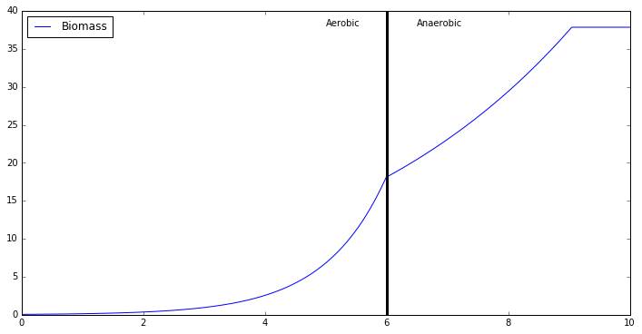
Here, let’s analyze data with an aerobic growth stage and anaerobic production stage.
In [1]:
import impact
import cobra
import cobra.test
# Hide some warnings to make the output cleaner
import warnings
warnings.filterwarnings('ignore')
% matplotlib inline
# Let's grab the iJO1366 E. coli model, cobra's test module has a copy
model = cobra.test.create_test_model("ecoli")
# Optimize the model
model.optimize()
# Print a summary of the fluxes
model.summary()
# Let's consider one substrate and five products
biomass_keys = ['Ec_biomass_iJO1366_core_53p95M']
substrate_keys = ['EX_glc_e']
product_keys = ['EX_for_e','EX_ac_e','EX_etoh_e','EX_succ_e']
analyte_keys = biomass_keys+substrate_keys+product_keys
# We'll use numpy to generate an arbitrary time vector
import numpy as np
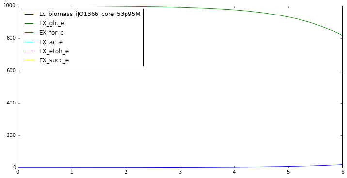
# The initial conditions (mM) [biomass, substrate,
# product1, product2, ..., product_n]
y0 = [0.05, 1000, 0, 0, 0, 0]
t_aerobic = np.linspace(0,6,600)
# Returns a dictionary of the profiles
from impact.synthetic_data import generate_data
dFBA_profiles_aerobic = generate_data(y0, t_aerobic, model,
biomass_keys, substrate_keys,
product_keys, plot = True)
# Let's make a new vector of initial values based on the output of the previous simulation
y0 = [dFBA_profiles_aerobic[analyte][-1] for analyte in biomass_keys+substrate_keys+product_keys]
C:\Users\Naveen\Anaconda3\lib\site-packages\IPython\html.py:14: ShimWarning: The `IPython.html` package has been deprecated. You should import from `notebook` instead. `IPython.html.widgets` has moved to `ipywidgets`.
  "`IPython.html.widgets` has moved to `ipywidgets`.", ShimWarning)
C:\Users\Naveen\Anaconda3\lib\site-packages\cobra\io\__init__.py:10: UserWarning:

cobra.io.sbml requires libsbml
IN FLUXES                     OUT FLUXES                    OBJECTIVES
o2_e        -17.58            h2o_e       45.62             Ec_biomass_iJO1366_core_53p95M    0.982
nh4_e       -10.61            co2_e       19.68
glc__D_e    -10.00            h_e          9.03
pi_e         -0.95            mththf_c     0.00
so4_e        -0.25            5drib_c      0.00
k_e          -0.19            4crsol_c     0.00
fe2_e        -0.02            meoh_e       0.00
mg2_e        -0.01            amob_c       0.00
cl_e         -0.01
ca2_e        -0.01
cu2_e        -0.00
mn2_e        -0.00
zn2_e        -0.00
ni2_e        -0.00
mobd_e       -0.00
cobalt2_e    -0.00
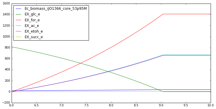
In [2]:
# Optimize the model after simulating anaerobic conditions,
# we don't get many products aerobically
model.reactions.get_by_id('EX_o2_e').lower_bound = 0
model.reactions.get_by_id('EX_o2_e').upper_bound = 0
model.optimize()
model.summary()

t_anaerobic = np.linspace(6,10,400)
dFBA_profiles_anaerobic = generate_data(y0, t_anaerobic, model,
                                        biomass_keys, substrate_keys,
                                        product_keys, plot = True)
IN FLUXES                     OUT FLUXES                    OBJECTIVES
glc__D_e    -10.00            h_e         27.87             Ec_biomass_iJO1366_core_53p95M    0.242
nh4_e        -2.61            for_e       17.28
h2o_e        -1.71            ac_e         8.21
pi_e         -0.23            etoh_e       8.08
co2_e        -0.09            succ_e       0.08
so4_e        -0.06            5drib_c      0.00
k_e          -0.05            glyclt_e     0.00
mg2_e        -0.00            mththf_c     0.00
fe2_e        -0.00            4crsol_c     0.00
fe3_e        -0.00            meoh_e       0.00
ca2_e        -0.00            amob_c       0.00
cl_e         -0.00
cu2_e        -0.00
mn2_e        -0.00
zn2_e        -0.00
ni2_e        -0.00
mobd_e       -0.00
cobalt2_e    -0.00
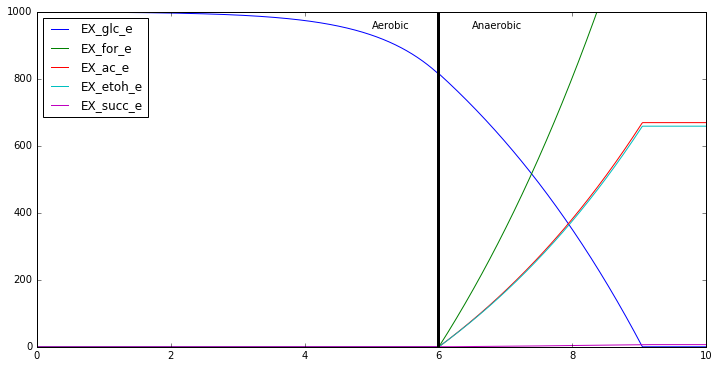
In [3]:
# Plot the whole profile
combined_profiles = {analyte:
                     dFBA_profiles_aerobic[analyte]+
                     dFBA_profiles_anaerobic[analyte]
                     for analyte in biomass_keys+substrate_keys+product_keys}

import matplotlib.pyplot as plt
% matplotlib inline
plt.figure(figsize=[12,6])
for analyte in substrate_keys + product_keys:
    plt.plot(np.linspace(0,10,1000),combined_profiles[analyte])
    min,max = plt.ylim()
    plt.ylim([0,max])

plt.text(5,max*0.95,'Aerobic')
plt.text(6+.5,max*0.95,'Anaerobic')
plt.legend(substrate_keys+product_keys,loc=2)
plt.plot([6]*10,np.linspace(min,max,10),'k',linewidth=3)

plt.figure(figsize=[12,6])
plt.plot(np.linspace(0,10,1000),combined_profiles[biomass_keys[0]])
min,max = plt.ylim()
plt.ylim([0,max])
plt.plot([6]*10,np.linspace(min,max,10),'k',linewidth=3)
plt.text(5,max*0.95,'Aerobic')
plt.text(6+.5,max*0.95,'Anaerobic')
plt.legend(['Biomass'],loc=2)
Out[3]:
<matplotlib.legend.Legend at 0x14d22326c50>
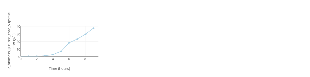
Now that we have a simulated ‘two-stage’ fermentation data, let’s try to analyze it. First let’s try to curve fit and pull parameters from the overall data
In [4]:
# These time courses together form a single trial
single_trial = impact.SingleTrial()
for analyte in analyte_keys:
    # Instantiate the timecourse
    timecourse = impact.TimeCourse()

    # Define the trial identifier for the experiment
    timecourse.trial_identifier.analyte_name = analyte
    timecourse.trial_identifier.strain_id = 'Demo'

    if analyte in biomass_keys:
        timecourse.trial_identifier.analyte_type = 'biomass'
    elif analyte in substrate_keys:
        timecourse.trial_identifier.analyte_type = 'substrate'
    elif analyte in product_keys:
        timecourse.trial_identifier.analyte_type = 'product'
    else:
        raise Exception('unid analyte')

    timecourse.time_vector = np.linspace(0,10,1000)
    timecourse.data_vector = combined_profiles[analyte]
    single_trial.add_titer(timecourse)

# Add this to a replicate trial (even though there's one replicate)
replicate_trial = impact.ReplicateTrial()
replicate_trial.add_replicate(single_trial)

# Add this to the experiment
experiment = impact.Experiment(info = {'experiment_title' : 'test experiment'})
experiment.add_replicate_trial(replicate_trial)

import plotly.offline
plotly.offline.init_notebook_mode()
fileName = impact.printGenericTimeCourse_plotly(replicateTrialList=[replicate_trial],
                                                titersToPlot=biomass_keys, output_type='image',)

from IPython.display import Image
Image(fileName)
Started fit
1000
Finished fit
This is the format of your plot grid:
[ (1,1) x1,y1 ]  [ (1,2) x2,y2 ]  [ (1,3) x3,y3 ]
Out[4]:
In [5]:
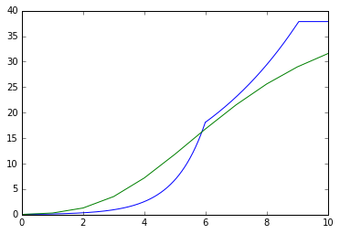
import matplotlib.pyplot as plt
for single_trial in replicate_trial.single_trial_list:
    print(replicate_trial.single_trial_list[0].analyte_dict[biomass_keys[0]].rate)
    plt.plot(np.linspace(0,10,1000),combined_profiles[biomass_keys[0]])
    plt.plot([0,1,2,3,4,5,6,7,8,9,10],replicate_trial.single_trial_list[0].analyte_dict[biomass_keys[0]].data_curve_fit([0,1,2,3,4,5,6,7,8,9,10]))
{'A': 38.794397885882105, 'lam': 5.4900330240132948, 'growth_rate': 4.9999996572528627}
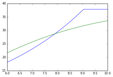
In [6]:
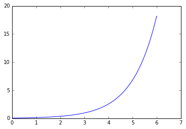
# We can break the trials into stages
replicate_trial.calculate_stages(stage_indices=[[0,600],[600,1000]])

for stage_number in [0,1]:
    print('Stage: ',stage_number)
    plt.figure()
    stage = replicate_trial.stages[stage_number]
    timecourse = stage.single_trial_list[0].analyte_dict[biomass_keys[0]]

    for single_trial in replicate_trial.single_trial_list:
        print(timecourse.rate)
        plt.plot(timecourse.time_vector,
                timecourse.data_vector)
        plt.plot(timecourse.time_vector,timecourse.data_curve_fit(timecourse.time_vector))

    plt.show()
[0, 600]
Started fit
601
Finished fit
[600, 1000]
Started fit
400
Finished fit
Stage:  0
{'A': 18.09275269452317, 'lam': 50.209771541246589, 'growth_rate': 3.0339841137990837}
Stage:  1
{'A': 38.794398023096186, 'lam': 4.4741197722850785, 'growth_rate': 4.9999859144920213}